Kezdőlap


Cím:	Harnessed Hazard
Szerző(k):	Cserti József
Füzet:	2004/januári melléklet, 48 - 57. oldal	PDF \| MathML

A szöveg csak Firefox böngészőben jelenik meg helyesen. Használja a fenti PDF file-ra mutató link-et a letöltésre.

To József Balog, my teacher at Károly Zipernowsky
secondary school

The Monte Carlo method

Chance has an extensive influence on everyday life. It is known to play an essential role in casinos, but besides that lots of random processes can be observed around us. (E.g., what direction does the fall of a pencil initially on its tip take?) Nature provides plenty of random processes as well. The gas atoms within a tank perform random motions. The decay of nuclei is another random process.
Chance can be used in the approximate determination of the value of

π

. Throw grains of rice (in a random way) on a square-shaped sheet of side

a

that has a circle of diameter

a

inscribed. Make

N

tries (counting only the attempts when the grains fall within the square), and count the number of grains in the circle (

N_{k}

). For large values of

N

(

N ≫ 1

), the ratio

N_{k} / N

gives a good approximation for the ratio of the areas of the circle and the square, that is

N_{k} / N = {(a / 2)}^{2} π / a^{2} = π / 4

. Thus, the value of

π

can be calculated as

π \approx 4 N_{k} / N

. Needless to say, this method does not lead to the precise value of

π

. However, the larger the number of tries, the more precise the result, as long as the grains fall onto the square in a uniformly random way.
Carrying out this real-life experiment is not necessary. A simple computer program will do the job, only a good random number generator is needed. Nowadays there are plenty of programs that can generate uniformly distributed random numbers on the unit interval

[0,1]

. Now generate a pair of them,

x

and

y

. This pair can be associated with a point in the first quadrant of the coordinate system (the position of the rice grain after the throw). If

x^{2} + y^{2} < 1

holds for the distance, then the point is within the unit circle. Suppose that the same algorithm is performed

N

times, and that the point falls within the circle

N_{k}

times. Just like in the case of the rice grains, the value of

π

is again approximated by the ratio

4 N_{k} / N

.
The table below contains the approximate values of

π

and their errors, obtained by increasing the number of tries. (The correct value of

π

to 9 decimal places is

π = 3.141 592 654

\begin{matrix} \begin{matrix} N & π & percentage error \\ 10 & 3.6 & 14.6 \\ 10^{2} & 3.16 & 0.6 \\ 10^{3} & 3.108 & 1.1 \\ 10^{4} & 3.127 & 0.5 \\ 10^{5} & 3.135 & 0.2 \\ 10^{6} & 3.141 & 0.02 \\ 10^{7} & 3.14155 & 0.001 \end{matrix} \end{matrix}

It is readily seen that for increasing

N

more and more precise values are obtained for

π

. A few hundred thousand attempts are sufficient for the correct determination of

π

to two decimal places. Nowadays computers perform over

10^{7}

tries within a minute. It is well worth the effort.
By means of completely random events, approximations have been obtained for a well-defined quantity. The above method can be carried further, and thus randomness can be used in the solution of extremely complex problems. The Monte Carlo method ‐ named after the famous casino in Monte Carlo ‐ is extensively used both in mathematics and physics. Metropolis and Ulam coined the name ``Monte Carlo'' in their 1949 article, mentioning that the random numbers necessary for the method could be taken from the results in a casino. In practice, random numbers are generated by computers themselves. Already in the beginning of the 20th century the method was used by a handful of statisticians, however its advent came with Neumann's, Ulam's and Fermi's attempts to obtain approximate solutions using computers for the complex mathematical problems of nuclear reactions.
Problems can very often be solved only by approximation methods. Luckily, very precise values are rarely needed. In such cases more often than not the Monte Carlo method proves very efficient. Below we will see some mathematical and physical examples for the application of the method. We tried to select problems that can be studied at the high-school level with today's computers.

Mathematical Applications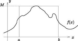

Figure 1. The area under the graph of the function

f (x)

on the interval

[a, b]

Determination of the area under a curve is a fundamental problem. The area

A

under the graph of function

f (x)

over the interval

[a, b]

(see Fig. 1) can be determined by dividing

[a, b]

N

equal sections of length

Δ x = (b - a) / N

, and approximating the area by the so-called rectangular sum: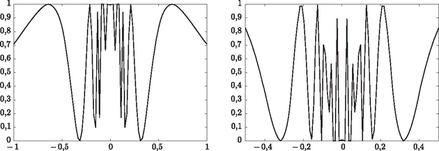

\begin{matrix} A \approx \sum_{i = 1}^{N} f (x_{i}) Δ x, \end{matrix}

where

x_{i}

is the midpoint of the

i

th subinterval. For simplicity assume that the function is positive on

[a, b]

, and let its maximum value on this interval be denoted by

M

. The larger

N

is, the more precise will the rectangular sum will be. This method is the most well-known (and also the simplest) way to determine the area under a curve. However, the function

f (x) = sin^{2} (1 / x)

‐ plotted in Fig. 2 ‐ oscillates very rapidly around the origin, so only excessively high values of

N

would ensure satisfactory precision in the determination of the area. The area under the graphs of rapidly oscillating functions can be efficiently approximated using the Monte Carlo method. Again, the method of throwing rice grains is applied. First, a random number

x

is generated (programming languages usually have a built-in random number generator that picks a random number from a uniform distribution over the unit interval

[0,1]

). Then this number is transferred into the interval

[a, b]

by means of the transformation

x \to a + x (b - a)

. Next, another random number

y

is generated, and transformed as

y \to y M

, leading to a (uniformly distributed) random number

y

in the interval

[0, M]

. Consider the two numbers as the coordinates

(x, y)

of a point. This point is inside the rectangle of sides

(b - a)

and

M

(see Fig. 1). If, in addition, the inequality

y < f (x)

holds for the coordinates

(x, y)

, then the point (grain of rice) is below the graph of

f (x)

Figure 2. Computer-generated graphs of the function

f (x) = sin^{2} (1 / x)

. Close to 0, the function oscillates violently, however, this is not shown in detail because of the ``finite resolution'' of the computer program. This is a purely numerical problem, which is not resolved by magnifying the centre part of the graph (see plot on the right)

Repeat the above sequence of operations

N_{total}

times, and count how many times the point is found under the graph. Let the number of such events be denoted by

N_{in}

. After a sufficiently large number of attempts,

N_{in} / N_{total}

is expected to give a good approximation for the ratio of the area

A

under the graph and that of the rectangle,

M (b - a)

, and so

\begin{matrix} A \approx M (b - a) \frac{N_{in}}{N_{total}} . \end{matrix}

Employ the above Monte Carlo method to the function in Fig. 2. The area under the graph over the interval

[a, b] = [0, b]

has been calculated, and the value of

b

has been varied between

0

and

1

. Values obtained by Monte Carlo calculations with different numbers of attempts are shown in Fig. 3. The areas are usually calculated using a well-known method of higher mathematics, integral calculus, which can be considered as the exact method. To illustrate the effectiveness of the Monte Carlo method, these exact values have also been plotted in the figures. For

N_{total} = 100

attempts the Monte Carlo method is seen to give a poor approximation of the exact result. However, for

N_{total} = 10,000

attempts the agreement is excellent with the exact result obtained by integration.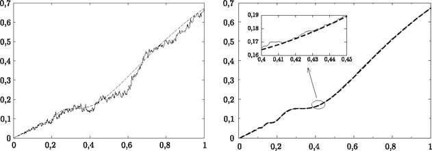

Figure 3. The area under the graph of

f (x) = sin^{2} (1 / x)

, obtained by the Monte Carlo method using

N_{total} = 100

(graph on the left) and

N_{total} = 10.000

(graph on the right) attempts. The dashed line shows the exact result

In what comes next, we will need area under the graph of the ``hat-like function''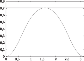

\begin{matrix} f (x) = sin^{2} (sin (x)) \end{matrix}

over the interval

[0, π]

, shown in Fig. 4. The Monte Carlo method using

\begin{matrix} N_{total} = 2^{22} = 4.194.304 \end{matrix}

attempts gives the result

A \approx 1.2194

, which agrees to three decimal places with the exact result

A = 1.2191

obtained by integration.

Figure 4. The ``hat-like function''. The maximum of the function on the interval

[0, π]

M = sin^{2} (1) = 0.7081

Physical Applications

In the first part of the article the basics of Monte Carlo methods have been presented, along with some simple mathematical applications. Physicists ‐ among others ‐ use this very method in a multitude of fields. Of the many physical applications, we will look at two below.

Determination of the centre of mass. High-school textbooks usually contain the method of determining the centre of mass. For some special geometries closed-form formulas can be given. (For example, the centre of mass of a semicircular sheet of uniform mass distribution is at a distance

4 r / 3 π

from the centre.) For more complicated shapes the position of the centre of mass is rather difficult to calculate; in general, the answer can only be given using integral calculus.
Consider, for example, the hat-like graph of Fig. 1 in Part I. For simplicity, we will only deal with reflection-symmetric plane figures. The symmetry axis of the hat-like function on the interval

[a, b] = [0, π]

is the vertical line

x = π / 2

, thus the horizontal coordinate of the centre of mass is evidently

π / 2

. An elementary calculation of the vertical coordinate is not possible.
In the general method, the figure is divided into several small strips of mass

m_{i}

; if the division is sufficiently fine, the vertical position of the centre of mass is given by the formula

\begin{matrix} y_{s} = \frac{\sum_{i}^{} y_{i} m_{i}}{\sum_{i}^{} m_{i}} . \end{matrix}

The denominator is proportional to the area of the figure. In the first part of the article, using the Monte Carlo method, the area of the hat-like function was found to be

A \approx 1.219

. The numerator can also be calculated with the same method. Generate two random numbers in the unit interval

[0,1]

x

and

y

. Transforming them according to

x \to x π

and

y \to M y

, the point with coordinates

(x, y)

will fall within a rectangle whose sides are

π

and

M

(where

M

, the maximum of the hat-like function is

M = sin^{2} (1) = 0.7081

). Then the numerator can be calculated using the following simple algorithm:

if (y < f(x) ) then
S = S + y
N_in = N_in + 1
endif

Applying the algorithm

N_{total}

times, the numerator in the previous formula can be approximated by

S M π / N_{total}

. Here

N_{in}

denotes the number of the points

(x, y)

under the graph

f (x)

. As we saw in the first part, the area

A

under the graph can be approximated by the expression

M π N_{in} / N_{total}

. Thus, the vertical coordinate of the centre of mass can be calculated from the formula

\begin{matrix} y_{s} = \frac{S}{N_{in}} . \end{matrix}

The variables

S

and

N_{in}

should be reset to zero at the beginning of each cycle. The program part above may, of course, need to be rewritten to comply with the rules of the chosen programming language. It is worth noting that the area under the graph is not a necessary input for the Monte Carlo calculation of the centre of mass.
Using integral calculus, the value

y_{s} = 0.274 975

is obtained, which can be considered exact. Fig. 5 shows the value of the centre of mass coordinate obtained with different numbers of attempts, as well as the exact value (dashed line). It is readily seen that for

N_{total} = 10^{6}

attempts the simulated value is in excellent agreement with the exact one (the relative difference is 0.02%).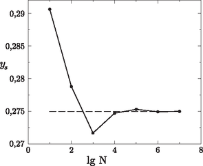

Figure 5. The centre of mass of the hat-like function, calculated by the Monte Carlo method. The dashed line shows the exact value

The Ising model. Certain materials exhibit magnetism. Loadstone (or magnesia stone) found around Magnesia, which attracts iron, was already known to the ancient Greeks. However, it was not until the 20th century, until the establishment of laws of quantum mechanics that the magnetic behaviour of these materials was satisfactorily explained. A model developed by Ising marked an important step in this research. In this simplified model the elementary magnets within the material (in our present view: the atomic spins) can be in each of two states: they can be parallel or antiparallel to the external magnetic field.
Imagine that the elementary magnets are placed in the vertices of a square lattice. The small magnet (spin) in the

i

th vertex of the lattice is aligned either parallel or antiparallel to the external field

H

, and so its value is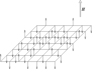

S_{i} = \pm 1

\begin{matrix} S_{i} = {\begin{matrix} 1, & if ↑ \\ - 1, & if ↓ . \end{matrix} \end{matrix}

A possible spin configuration is shown in Fig. 6. Each elementary magnet ``feels'' the instantaneous direction of the other magnets, that is, the spins interact. In this model only interactions between nearest neighbours (or: first neighbours) are taken into account, and the effects of magnets separated by larger distances are neglected. Thus, there is a spin in each lattice site that interacts with its four nearest neighbours. The spins tend to align themselves parallel to the external magnetic field

H

. With the above interactions, the total energy

E

of the system can be written as

\begin{matrix} E = - J \sum_{〈 i, j 〉}^{} S_{i} S_{j} - H \sum_{i}^{} S_{i}, \end{matrix}

where

J

, usually called the coupling constant, is a number characteristic of the strength of the interaction between adjacent spins. In the first term, the sum is over first neighbours only;

〈, 〉

is the shorthand notation for this.

Figure 6. The Ising model of spin systems. The spins are either parallel or antiparallel to the external magnetic field

H

The magnetisation

M

of the system is the sum of all spin variables (or proportional to this quantity),

\begin{matrix} M = \sum_{i}^{} S_{i} . \end{matrix}

Imagine that the system is cooled to absolute zero, and the external field is switched off. The system is now in its ground state (its lowest energy state, in other words: its ``energetically most favourable'' state). If the coupling constant

J

is positive, then all spins are aligned in the energetically favourable state (since the product of neighbouring spins is

+ 1

in this state), so the arising state is magnetically ordered. In the ground state (for

J > 0

) the magnetisation of the system is maximal. This is the ferromagnetic state.
As the temperature is increased, more and more spins ,,flip'' into the opposite direction, and so the magnetisation of the system decreases. Above a certain temperature

T_{c}

‐ in the absence of an external magnetic field ‐ on average half are aligned upwards, and the other half downwards; the magnetisation

M

is thus zero. This temperature is called the critical temperature or the Curie temperature, named after the French physicist Pierre Curie. Even in the absence of a magnetic field

H

the ordered state is completely destroyed at increasing temperatures. The magnetisation of the system has a finite (non-zero) value below

T_{c}

, while it vanishes for temperatures exceeding it. This phenomenon ‐ along with the changes in the state of matter, similar in many respects ‐ belongs to the class of phase transitions. Even with this simple model it can be understood why a magnet loses its magnetisation when thrown into fire. The temperature dependence of magnetisation is sketched in Fig. 7.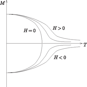

Figure 7. temperature dependence of the magnetisation in the Ising model, in the presence of different external magnetic fields

It is worth noting that the coupling constant

J

can be negative as well; in this case, and if the magnetic field is zero, the neighbouring spins are antiparallel (their product is

- 1

) in the ground state, and a checkerboard-like structure is formed. Nature provides many examples of such antiferromagnetic systems.
Below, we will present an algorithm based on the Monte Carlo method that can be used to determine how the magnetisation of the system shown in Fig. 3 depends on the temperature and the external magnetic field. The algorithm was first applied to spin systems by the Greek-American mathematician N. Metropolis half a century ago, and has been called Metropolis algorithm ever since [1]. The spins are thought to be arranged in a square lattice, according to Fig. 2, and periodic boundary conditions are applied. This means that the entire square lattice is thought to be periodically repeated indefinitely in the directions of its sides, or, alternatively, the lattice is drawn onto a torus (the surface of a doughnut). This trick ensures that the spins originally at the edge of the square have four nearest neighbours, and so they are no longer different from those inside the lattice.
Consider some initial spin configuration ‐ for example the ordered ground state corresponding to zero temperature. Then, the following steps are repeated:

1	A spin is chosen randomly. The change in the energy of the system due to flipping over this spin is calculated; this quantity will be denoted by $Δ E$ .

The probability that the chosen spin flips over at temperature

T

is calculated. This probability (the so-called transition probability) can be calculated as

\begin{matrix} W = {\begin{matrix} 1, & if Δ E < 0 \\ e^{\frac{Δ E}{k T}}, & if Δ E > 0, \end{matrix} \end{matrix}

where

k

is the Boltzmann constant.

3	A random number $r$ is generated on the interval $[0,1]$ . If $r < W$ , then the spin in question is flipped, otherwise it is left unaltered.

4	Back to step 1.

It can be shown that after sufficiently many cycles of the above algorithm the magnetisation settles at an equilibrium value

〈 M 〉

that is determined by the temperature

T

and the external magnetic field

H

. A certain number of iterations (time) is always necessary to reach the equilibrium state. This time, denoted by

T_{rel}

, is called the relaxation time, and is usually counted in Monte Carlo steps (MCS). One MCS is the time necessary to chose each spin once for the iteration step on the average. Fig. 8 shows the typical dependence of magnetisation on time (the number of cycles).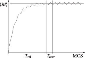

Figure 8. The time dependence of the magnetisation during the iterations, in MCS units

The relaxation time can be determined empirically. If the magnetisation

M

does not change significantly and just fluctuates slightly, then the equilibrium state has been reached. Then the average magnetisation

〈 M 〉

can be determined by calculating the magnetisation with a certain frequency, and taking the average of the results. If the temperature is varied and the behaviour of the magnetisation is studied, then the ``measurements'' can provide data for the temperature dependence of the magnetisation.
The behaviour of the infinite, two-dimensional Ising model with zero external magnetic field was first calculated analytically (i.e. without approximations, in closed form) by L. Onsager [2]. The critical temperature of this system is

k T_{c} = 2.27 J

. In the light of the exact solution, the precision of the Monte Carlo method can be studied. To date, no analytical method has been found in three dimensions (i.e. for spatial lattices), however, such systems have also been studied extensively using the Monte Carlo method.
When applying the Monte Carlo method, attention should be paid to the possible sources of error. For example, because of the finite size of the system, the critical temperature for planar lattices does not agree with the known theoretical value. In this case the dependence of the critical temperature on the lattice size must be examined, with the aim of extrapolating to the infinite system.
Another frequent problem is having a ``good'' random number generator. Sometimes the successive numbers of the generator are not completely independent of each other; this inevitably leads to incorrect results. Testing the random number generator is therefore essential.
Some problems that are easy to program can be found in reference [3].

I wish to thank my colleagues, János Kertész and Tamás Vicsek for familiarizing me with the Monte Carlo method, Tamás Geszti and Péter Pollner for their useful advice, and my students, János Koltai, Szilárd Pafka and József Szűcs for their help in this work.

References and Suggested Reading

[1]	N. Metropolis, A. W. Rosenbluth, M. N. Rosenbluth, A. H. Teller and E. Teller, J. Chem. Phys., 21 (1953), 1087.

[2]	L. Onsager, Phys. Rev., 65 (1944), 117.

[3]	J. Kertész, J. Cserti and J. Szép: Monte Carlo simulation programs for microcomputer, Eur. J. Phys., 6 (1985), 232.